Several weeks ago, I was asked a question by another investor, if we couldn’t use mean-variance in our portfolio building process, what would we use?
The question stumped me somewhat, as while I’d done some research into adapting mean-variance optimisation and am aware of the input variable issues, I wasn’t entirely sure there would be some unknown strategy that might be worth considering.
I turned the question into today’s morning note to explore some of the pitfalls of modern asset allocation.
The most common approach to building a multi-asset portfolio is to choose the portfolio with the highest expected return for a specific degree of risk.
This risk quotient will vary client-to-client, mandate-to-mandate, objective-to-objective, where different client or client sets will have different risk appetites and risk aversion functions.
This particular blend of risk and return was first postulated by Harry Markowitz and is now known as “Modern Portfolio Theory”, or the E-V Maxim, where portfolios are constructed to provide the highest (expected) return for a given level of (expected) risk.
Portfolios that sit along this frontier are deemed to be “efficient”, where an efficient portfolio is the optimal mix between risk and return, where the gradient of the capital market line is the client’s risk aversion.
In practice, we’re building portfolios that have the best Sharpe Ratios, and treating both upside and downside volatility as the same.
For example, wanting $0.8 return for $1 of risk (both good and bad volatility/risk), when the risk-free rate is 3% p.a., we would build a line that intercepts the Y-axis at 3% and draw tangentially at this gradient of 0.8.
Chart 1: Efficient Portfolio Frontier
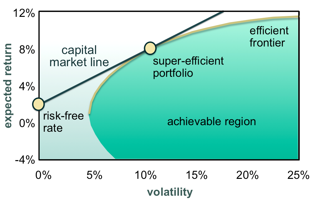
Source: Schoenmaker and Schramade 2020
In practice, there are three key input variables used to derive an E-V maxim:
- Expected return
- Expected risk (variance)
- Expected correlation
Together, these inputs can be transformed into a co-variance matrix, where we can begin to rank asset classes by their risk and return expectations.
The below is a simple co-variance table that I’ve drawn up to highlight this process, where my expected return for stocks is 10% and for bonds 8% (hey, we can dream right?), the expected risk is known (or hedged) at 20% and 10% appropriately, and correlation between the two investment instruments is 50%.
From there we can play around with the percentage allocation between stocks and bonds to derive the marginal utility each asset class provides a portfolio, where at 2/3 bonds and 1/3 stocks our marginal utilities are equal, and thus the trade-off between adding additional bonds or additional stocks is the same.
Table 1: Marginal Effect of Varying Asset Class Weights
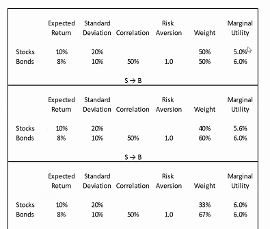
Source: Mason Stevens
From there we can add some more sexy visualisation and start to depict what a portfolio will grow or shrink to, over time, based on these forward-looking assumptions.
The below is a chart I’ve taken from our Mason Stevens Investment Platform, where clients can see this visualisation themselves, based on our in-house market assumptions for each asset class.
This generic account holds 3.4million AUD spread across domestic and international equities, fixed income, property, and infrastructure exposure, with confidence bands at the 30th, 60th and 90th percentiles.
Chart 2: Mason Stevens’ Portfolio Projections Tool
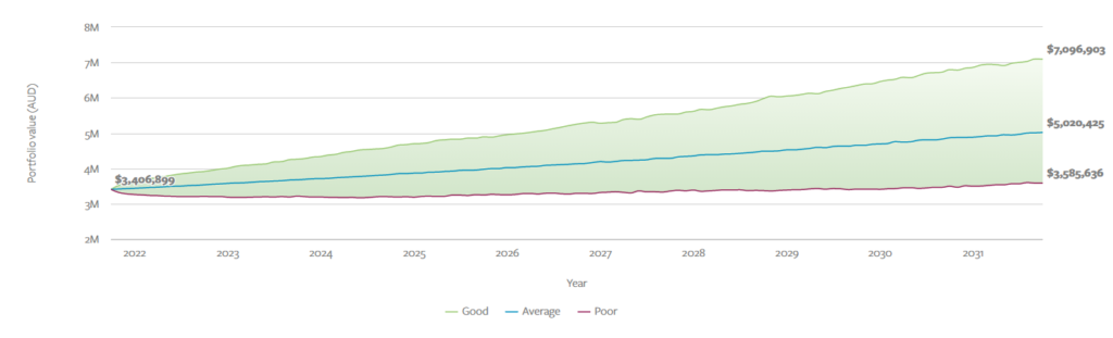
Source: Mason Stevens
Input Errors
The problem with this methodology is that the input variables of return, risk, and correlation can be misleading, where if they are deviant from reality, the effect will be magnified over several years due to the compounding nature of economic returns.
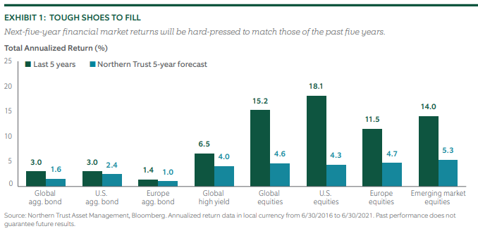
Taking for example the capital market assumptions produced by global asset manager Northern Trust in 2016, with a 5-year outlook, it was far from consensus that US equities would perform so well on both an absolute and relative return basis.
Moreover, the equity risk premia of “growth” continued to outperform “value” over this time period, where many had forecast for a mean-reversion style of correction, where value had underperformed for several years already prior to 2016.
Likewise, if you had told most strategists and portfolio managers in 2019 when the yield curve inverted, that in 2020 we’d have a recession, not many would’ve suggested that we would’ve seen the equity market enter a strong bull market rally within two months and finish well up on the year.
Hence, Northern Trusts’ forecast (blue bars) for equity returns had a marked differential to the realised performance (green bars).
Chart 3: Northern Trust’s 2016 5-year Forecast Vs Actual Results
And this isn’t limited to return as well, our correlation and risk assumptions may also be far from realistic, regardless of if we use backward-looking or forward-looking assumptions.
Myself, I always look forward to the 7-year forward-looking returns that Grantham, Mayo, van Otterloo (GMO) produce, which highlight based on their assumptions, nearly all asset classes will perform poorly on an annualised basis, going forward to 2028.
Where for example, US large-cap equities are predicted to return an average -8% each year, for the coming 7 years.
Chart 4: GMO 7-year Forecast
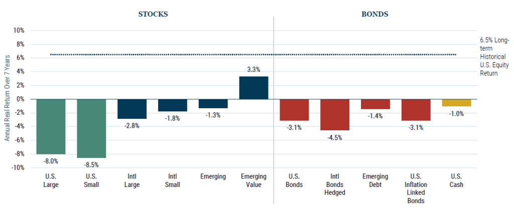
Source: GMO
Tail-Risk
Part of the problem with input errors or assumption biases is that asset class returns tend not to be normally distributed, where they have “fat tails”, referring to times when returns are deeply positive or negative, several standard deviations from the arithmetic mean return.
Visually, these would be events that are greater than +/- 3 sigma, or the far left or right of the below distribution.
This is known as “skewness”, and is similar to the concept of disaster insurance, where the insurer collects many small premiums (returns) and wants to limit the amount of overly large payouts required to the insured party (losses).
Chart 5: Normality Distribution
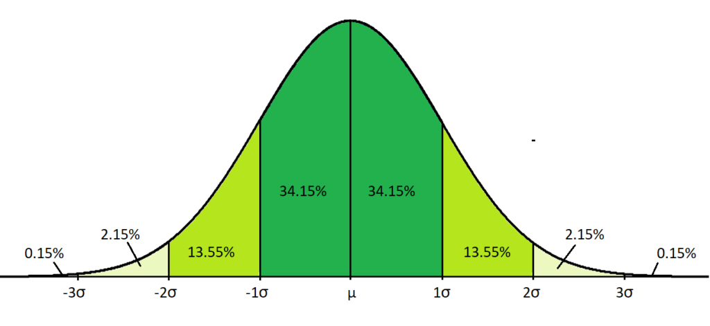
Source: Curtin University
To complicate the matter slightly more, asset class returns tend to be positive over longer periods of time, which is why some will ignore short-term price gyrations and market volatility, in favour of building long-term portfolios that have assets mostly in the top right quadrant of returns.
The below chart compares US equity returns versus emerging market equities, over a 20-year period.
Chart 6: US versus EM Equity Correlations, 10-20y Time Horizon
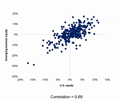
Source: MIT
If we ran the same analysis again but for the 3-year period between 2017-2020, the result would starkly different.
Chart 7: US versus EM Equity Correlations, 3y Time Horizon
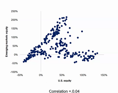
Source: MIT
This highlights an inherent flaw that mean-variance analysis cannot accommodate skewed distributions or non-quadratic functions unless investor preferences are fully described in our capital market line (the trade-off between risk and return), where likely, they aren’t.
Quadratic Utility
Most plausible utility functions are upward sloping, which implies that more wealth is preferable compared to less.
Quadratic (power) utility functions fit this brief for the most part, though some investors may have “kinked” utility, representing a sharp dissatisfaction with returns below some specific level, where the relationship can’t be solely described by expected return and risk.
Chart 8: Kinked and S-Shaped Utility Functions
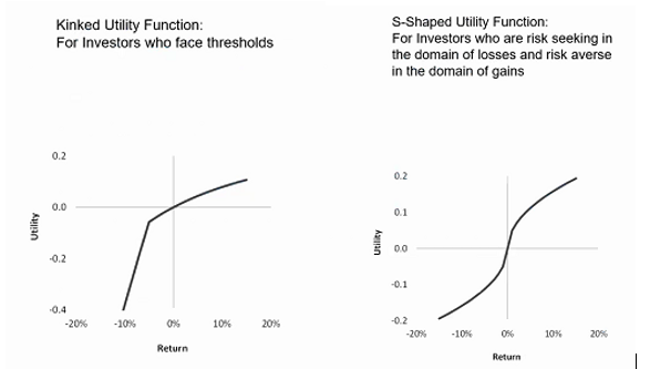
Kinlaw, Kritzman, Turkington (2017)
Alternative Approaches
In trying to accommodate the known issues with mean-variance (input errors, skewness, and non-quadratic utility functions), there are several approaches that can be utilised.
To combat the problems associated with input assumptions, we can utilise a “minimum variance” approach to minimise the price volatility of the overall portfolio, where, unfortunately, we still have the same issues of skewness and non-quadratic utility.
However, min-variance is useful for more conservative portfolios, where in practice you tend to build a portfolio with a low volatility instruments (think cash, fixed income) or having few volatile instruments which have low correlation with one another (direct lending, RMBS, EM sovereign debt, etc), balanced with an investment-grade fixed income or enhanced cash allocation for income.
The problem with min-variance is that we tend to build similar portfolios to mean-variance, where for conservative portfolios they tend to be dominated by income generation rather than capital growth, and where Sharpe Ratios are fairly accurate as a prescription of risk budgeting, compared to say a growth portfolio that might need to cater for downside volatility.
You could also think of this as a form of “risk budgeting”, where the amount of possible volatility is distributed in a budget-like fashion within a portfolio, where for example stocks could be given a risk budget of 10% with a hedge put in place for anything further, optimised with fixed income which tends to have known volatility +/- 2-3%.
Another approach is called “risk parity”, a more advanced technique that allows for leverage (borrowing), as well as short selling in portfolios and funds.
Following this approach, allocators don’t simply generate the optimal mix of assets the way they do under mean-variance, the optimiser also uses leverage and long/short exposure to weight risk equally among different (and possibly more) assets, using an optimal risk budget.
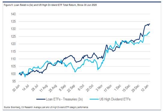
To illustrate this point, Citi published a research paper on 19-Jan-2021 comparing senior bank loan ETFs to equity income (dividend) strategies.
What they found was that senior loan ETFs are 3-4x less volatile than equity income strategies, where their returns are not 3-4x less.
Under risk-parity, investors would be better suited to use leverage to buy senior loan ETFs than to simply invest in the equity income strategy – assuming the same amount of exposure.
Chart 9: 3x Levered Senior Bank Loan ETFs Outperform High Dividend ETFs
For situations where we believe returns are not elliptically distributed and preferences are non-quadratic, we tend to resort to a technique called “full-scale optimisation”, which is conceptually straightforward but computationally intensive.
What we do is run scenario analysis (simulations) across all permissible sets of portfolio weights and select whichever combination produces the highest expected utility.
For example, this is how many simulations we would need to run, to build a fully scaled portfolio with growing number of asset or asset classes, with small weight increments.
Table 2: Computation Requirements for Full Scale Optimisation by Input Variable
| Number of Assets | Weight Increment | Number of Possible Portfolios |
| 2 | 5.00% | 21 |
| 7 | 5.00% | 230,230 |
| 7 | 2.50% | 9,366,819 |
| 14 | 5.00% | 573,166,440 |
| 14 | 2.50% | 841,392,966,470 |
| 28 | 5.00% | 9,762,479,679,106 |
| 28 | 2.50% | 4,105,075,349,580,980,000 |
| 28 | 1.25% | 15,738,530,963,776,300,000,000,000 |
Source: Mason Stevens
Computers have become much better since 1952 when Markowitz penned Modern Portfolio Theory, but they aren’t quite fast enough yet to run that many simulations in any time frame that helps build investment portfolios.
Conclusions
Mean-variance has withstood the test of time these past six decades, where if we can reasonably approximate expected return and expected risk, where investors have quadratic utility preferences, we can build an optimal portfolio for their use.
However, if we find we can’t reasonably approximate any of the key input variables required, there are techniques available to us to fall back upon, with differing efficacy in approach and skill required to implement.
References:
C. Jarque and A. Bera (1980), “Efficient tests for normality, homoscedascity and serial independence of regression residuals”, Economics Letters, Vol. 6, No. 3.
H. Markowitz and K. Blay (2014), “The Theory and practice of Rational Investing: Risk-Return Analysis”, Volume 1, McGraw Hill
W. Kinlaw, M.P. Kritzman, D.Turkington (2017) “A Practioners Guide to Asset Allocation”, Wiley (New Jersey)
M.D. Braga (2016), “Alternative Approaches to Traditional Mean-Variance Optimisation”, Asset Management and Institutional Investors, pp.203-13, ResearchGate
The views expressed in this article are the views of the stated author as at the date published and are subject to change based on markets and other conditions. Past performance is not a reliable indicator of future performance. Mason Stevens is only providing general advice in providing this information. You should consider this information, along with all your other investments and strategies when assessing the appropriateness of the information to your individual circumstances. Mason Stevens and its associates and their respective directors and other staff each declare that they may hold interests in securities and/or earn fees or other benefits from transactions arising as a result of information contained in this article.
